
Hello! In this blog post, I'll be talking about the Big O notation section from the first chapter of Grokking Algorithms. The book makes it really easy to understand what Big O notation is and how it helps us determine the efficiency of an algorithm.
TL;DR
- Big O notation tells you how fast an algorithm is with large amounts of data using math that looks like this:
"Big O" -> O(n) <- "Number of Operations"
Simple search has a runtime of
O(n)that's also known as linear time.In a list of 100 numbers where you're trying to find one. This runtime steps through each until you find the correct one
Binary search on the other hand halves the list repeatedly while determining which half the number is in reduces the time it takes to find that number. The runtime of this is
O(log n)known as logarithmic time.
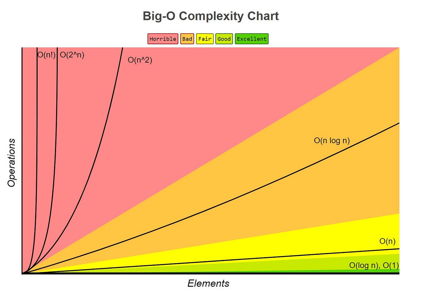
Here are the common runtimes and how they compare when introduced to big amounts of data:
- O(log n), also known as logarithmic time. Example: binary search.
- O(n), also known as linear time. Example: simple search.
- O(n * log n). Example: a fast sorting algorithm, like quicksort.
- O(n^2), or n to the power of 2. Example: a slow sorting algorithm, like selection sort.
- O(n!). Example: a very slow algorithm, like the traveling salesperson problem.
In other words, algorithms go BRR and binary search is supa FAST!
(Insert Initial D song YouTube song link )

What is Big O Notation?
The book explains that "Big O notation is special notation that tells you how fast an algorithm is." The author also mentions "runtime," which refers to how quickly an algorithm completes a task depending on the size of the input.
What is this special notation? The author gives an example of the notation as:
"Big O" -> O(n) <- "Number of Operations"
This tells you the number of operations an algorithm will take, and it's called "Big O" because you put an uppercase "O" in front of the number of operations.

O of n O(n), where n is the number of elements, means there will be as many operations as there are elements. The worst-case scenario is used when determining how long an algorithm will take.
Simple Search vs Binary Search Growth Rates
The book gives us an example where bob is comparing two algorithms with a list of 100 elements. One of the algorithms we use is simple search and it has a runtime of O(n). This runtime is known as linear time. The algorithm will look at each element until it finds the one we are looking for. In the worst-case scenario, we could look through 99 names in the list.
Comparing this to binary search, which halves the list repeatedly while determining which half the name is in, significantly reduces the time. The runtime for binary search is O(log n). Also known as logarithmic time.
The author gives each operation a time of 1ms. Simple search will take 100ms while binary search will take 7ms only having to guess 7 times. When the list of elements grows the times drastically change. Here's the comparison that's included in the book:
| # of Elements | Simple Search | Binary Search |
|---|---|---|
| 100 | 100ms | 7ms |
| 10,000 | 10 seconds | 14ms |
| 1,000,000,000 | 11 days | 30ms |
Another example that's given is having to draw squares on a piece of paper. Using a pencil to draw 16 squares one at a time takes O(n), but folding the paper in half repeatedly let's you draw twice as many boxes than drawing one at a time.
Comparing Runtimes
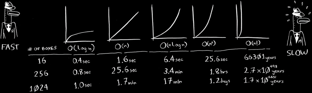
In the last bit of the section the author talks about having to do the squares on paper example with different runtimes.
Here's a list of the common runtimes the book talks about from fastest to slowest:
- O(log n), also known as logarithmic time. Example: binary search.
- O(n), also known as linear time. Example: simple search.
- O(n * log n). Example: a fast sorting algorithm, like quicksort.
- O(n^2), or n to the power of 2. Example: a slow sorting algorithm, like selection sort.
- O(n!). Example: a very slow algorithm, like the traveling salesperson problem.
Here's an example of how each runtime performs that's included in the book:
Here's an image of the runtimes compared on a chart that might make it a bit more clear:
I hope this dive into a section of grokking algorithms convinces you to get the book and further explore what it has to offer. I've been enjoying it so far. If you have any feedback please reach out to me on my Linkedin here: My Linkedin
Grokking Algorithms Second Edition
Thanks for reading!
